DeepLearning from Scratch - Ch3. Neural Network
[review]
Perceptron
- pros: variety of complex processes can be solved with perceptrons
- cons: user have to choose parameters(weight, bias) him/herself.
Neural Network can solve this problem. It can automatically train proper parameters from data itself.
3.1 Perceptron to Neural Network
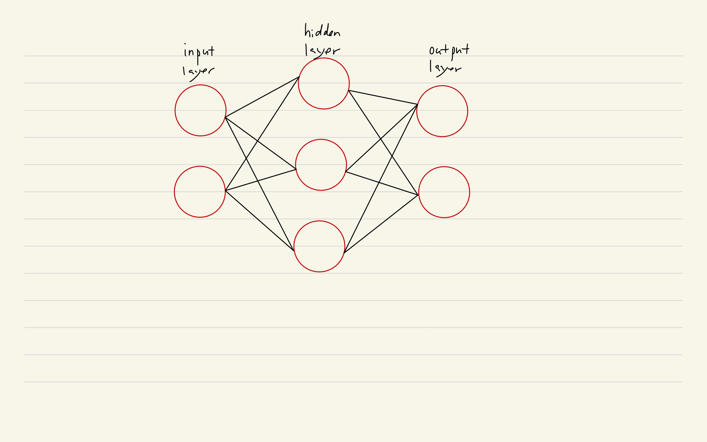
Perceptron and Neural Network looks similar.
- The main difference is in activate function.
- Perceptron uses step function as activate function.
- Neural network uses sigmoid, ReLU, tanh etc.
3.2 Activation Function
- We can separate this perceptron’s eqation.
activation function
- $h(x)$ above is called activation function.
- This convert sum of all the input signals to output signals.
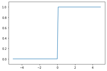
3.2.1 Step Function
- From the example above($h(x)$), Output is determined by threshold. This function is called step function.
excercise of float number
import numpy as np
# cf) np.array can be written in inequality but list can't be

a = np.array([1.2, 0.2, -0.1])
a > 0
array([ True, True, False])
b = [1.2, 0.2, -0.1]
b > 0
---------------------------------------------------------------------------

TypeError                                 Traceback (most recent call last)

<ipython-input-3-2322d757a24f> in <module>
      1 b = [1.2, 0.2, -0.1]
----> 2 b > 0


TypeError: '>' not supported between instances of 'list' and 'int'
step function
def step_function(x):
    # cf) x only can get float type, not numpy array
    if x > 0:
        return 1
    else:
        return 0
print(step_function(1.2))
print(step_function(-0.7))
1
0
def step_function(x):
    y = x > 0
    # use astype method to convert numpy array
    return y.astype(np.int)
step_function(np.array([-1.0, 1.0, 2.0]))
array([0, 1, 1])
3.2.2 Step Function Graph
import matplotlib.pyplot as plt

def step_function(x):
    return np.array(x > 0, dtype=np.int)

x = np.arange(-5.0, 5.0, 0.1)
y = step_function(x)

plt.plot(x,y)
plt.ylim(-0.1, 1.1)
plt.show()
3.2.3 Sigmoid Function
def sigmoid(x):
    return 1/(1+np.exp(-x))

x = np.array([-1.0, 1.0, 2.0])
sigmoid(x)
array([0.26894142, 0.73105858, 0.88079708])
x = np.arange(-5, 5, 0.1)
y = sigmoid(x)

plt.plot(x,y)
plt.ylim(-0.1, 1.1)
plt.show()
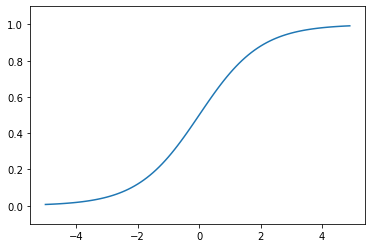
3.2.4 Step Function VS Sigmoid Function
Both of them are nonlinear function. However, output differs.
- The output of step function is discrete (0 or 1)
- The output of sigmoid function is continuous (0 ~ 1)
3.2.5 Nonlinear Function
In neural network, we should not use linear function as a activation function.
The problem of linear function is here.
- The combination of linear function is also linear. - As we saw at Chapter 2, we cannot solve complicated problems with one linear line.
The strength of neural network is in deep density of hidden layer. However if the activation function is linear, it will be useless to make deep hidden layers.
Ex) \(\begin{cases} h(x) = cx\\ y(x) = h(h(h(x))) = c^3x\end{cases}\)
3.2.6 ReLU(Rectified Linear Unit)
ReLU
\[h(x) =\begin{cases} x \;\;(x>0)\\ 0 \;\;(x\leq0)\end{cases}\]def relu(x):
return np.maximum(0,x)
# np.max([1,2,3,4]) = 4 : choose the maximum value in list/array
# - one input data
# np.maximum([1,2,3], [4,5,6]) = [4,5,6] : choose the list/array that has maximum element
# - two input data with same shape
# - if two scalar given, choose maximum value
relu(3)
3
3.3 Ndarray
a = np.array([1,2,3])
a.shape
a.ndim
1
b = np.array([[1,2], [3,4], [5,6]])
b.shape
(3, 2)
There is no difference between row vector, and column vector.
- They are treated same when multiplying
a = np.array([1,2])
b = np.array([[1,2], [3,4], [5,6]])
c = np.array([[1,2,3], [4,5,6]])

print(a.dot(c))
print(b.dot(a), end='\n\n')

print(a.T.dot(c))
print(b.dot(a.T))
[ 9 12 15]
[ 5 11 17]

[ 9 12 15]
[ 5 11 17]
3.4 Neural Network
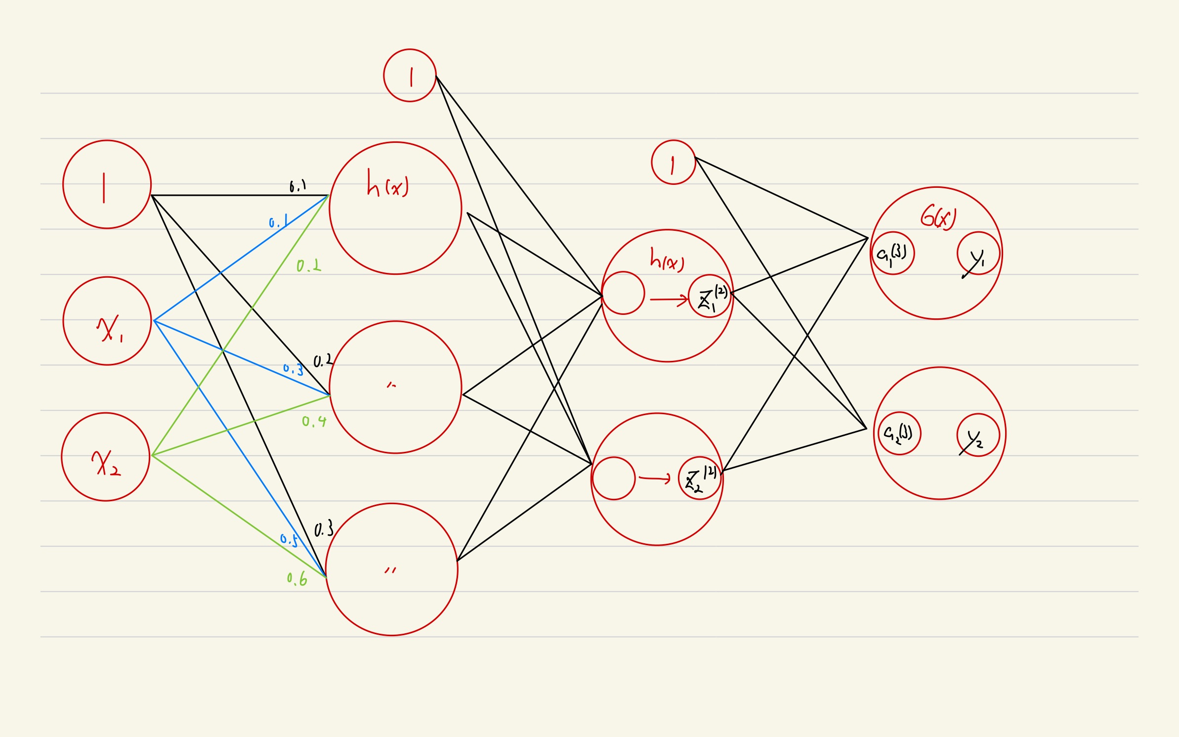
- $h(x)$ is activation function.
- $\sigma()$ is activation function on the output layer.
- $\sigma()$ differs
- here, we use identity function
- regression: identity function
- classification: softmax function
# output layer step function
def identity_function(x):
    return x

# dictionary of weight and bias
def init_network():
    network = {}
    network['W1'] = np.array([[0.1, 0.3, 0.5], [0.2, 0.4, 0.6]])
    network['b1'] = np.array([0.1, 0.2, 0.3])

    network['W2'] = np.array([[0.1, 0.4], [0.2, 0.5], [0.3, 0.6]])
    network['b2'] = np.array([0.1, 0.2])

    network['W3'] = np.array([[0.1, 0.3], [0.2, 0.4]])
    network['b3'] = np.array([0.1, 0.2])

    return network

# neural network
def forward(network, x):
    W1, W2, W3 = network['W1'], network['W2'], network['W3']
    b1, b2, b3 = network['b1'], network['b2'], network['b3']

    a1 = np.dot(x, W1) + b1
    z1 = sigmoid(a1)

    a2 = np.dot(z1, W2) + b2
    z2 = sigmoid(a2)

    a3 = np.dot(z2, W3) + b3
    y = identity_function(a3)

    return y

network = init_network()
x = np.array([1.0, 0.5])
y = forward(network, x)

print(y)
[0.31682708 0.69627909]
3.5 output layer : $\sigma()$
3.5.1 Softmax Function
softmax function
\[y_k = {exp(a_k)\over \sum_{i=1}^{n}{exp(a_i)}}\]- $n$: # of neurons in the output layer
- $y_k$: k-th output
def softmax(a):
    exp_a = np.exp(a)
    sum_exp_a = np.sum(exp_a)
    y = exp_a / sum_exp_a

    return y

a = np.array([0.3, 2.9, 4.0])
print(softmax(a))
[0.01821127 0.24519181 0.73659691]
3.5.2 Features of Softmax Function
- The output is continuous value between 0 and 1
- Sum of all the values are 1
- It can be interpreted as probability
- Neuron with highest result is selected as output class
- Order relation is same as before softmax calculation
- reason: $e^x$ is monotone increasing function
- Because of calculation time efficiency, usually skip softmax process in field work.
3.5.3 Choosing output numbers.
In classification problem, the number of neurons is same as the number of classes.
3.6 Practice with MNIST Datasets
# Unlike the lecture, I used keras mnist datasets
from tensorflow.keras.datasets import mnist
# python image library
from PIL import Image

def img_show(img):
    pil_img = Image.fromarray(np.uint8(img))
    pil_img.show()

# ((train_img, train_label), (test_img, test_label))
((x_train, y_train), (x_test, y_test)) = mnist.load_data()

print(x_train.shape, x_test.shape)
print(y_train.shape, y_test.shape, end='\n\n')

# preprocessing mnist datasets : flatten
x_train = x_train.reshape(60000, 28 * 28)
x_test = x_test.reshape(10000, 28 * 28)

img = x_train[0]
label = y_train[0]
print(label, end='\n\n')

print(img.shape)
img = img.reshape(28,28)
print(img.shape)

img_show(img)
(60000, 28, 28) (10000, 28, 28)
(60000,) (10000,)

5

(784,)
(28, 28)
3.6.2 Neural Network Prediction
import pickle

# not normalized data
def get_data():
    ((x_train, y_train), (x_test, y_test)) = mnist.load_data()

    x_train = x_train.reshape(60000, 28 * 28)
    x_test = x_test.reshape(10000, 28 * 28)

    return x_test, y_test

# trained parameter dictionary
# pickle file on "asset -> files" directory
def init_network():
    with open('sample_weight.pkl', 'rb') as f:
        network = pickle.load(f)

    return network

def prediction(network, x):
    W1, W2, W3 = network['W1'], network['W2'], network['W3']
    b1, b2, b3 = network['b1'], network['b2'], network['b3']

    a1 = np.dot(x, W1) + b1
    z1 = sigmoid(a1)
    a2 = np.dot(z1, W2) + b2
    z2 = sigmoid(a2)
    a3 = np.dot(z2, W3) + b3
    y = softmax(a3)

    return y
x, y = get_data()
network = init_network()

accuracy_cnt = 0
for i in range(len(x)):
    y_pred = prediction(network, x[i])

    # get label with highest probability
    p = np.argmax(y_pred)

    if p == y[i]:
        accuracy_cnt += 1

print('Accuracy : ', float(accuracy_cnt)/len(x))
/opt/anaconda3/lib/python3.7/site-packages/ipykernel_launcher.py:2: RuntimeWarning: overflow encountered in exp


Accuracy :  0.9207
3.6.3 batch
x, y = get_data()
network = init_network()

batch_size = 100
accuracy_cnt = 0

for i in range(0, len(x), batch_size):
    # 0~99 / 100~199 / ...
    x_batch = x[i:i+batch_size]
    y_batch = prediction(network, x_batch)

    p = np.argmax(y_batch, axis=1)

    accuracy_cnt += np.sum(p == y[i:i+batch_size])

print('Accuracy : ', float(accuracy_cnt)/len(x))
Accuracy :  0.9207


/opt/anaconda3/lib/python3.7/site-packages/ipykernel_launcher.py:2: RuntimeWarning: overflow encountered in exp