DeepLearning from Scratch - Ch4. Neural Network Learning

8 minute read

4.1 Learning From Data

What is learning?

Learning is to get optimal parameters from train data
Our aim is to minimize Loss Function which shows whether training process is successfully working

Machine Learning

Data is important element in Machine Learning
Machine Learning finds patterns from data

Let’s say we aim to classify mnist data. There are 3 ways of finding pattern.

Find Pattern and make a logic
Extract features from image(=data) and use machine learning method
- We have to convert these features into vectors ourself
- Here, Feature Engineering is important
Use Neural Network(Deep Learning) skills
- NN(DL) also learns important features itself
- DL is also called end-to-end Machine Learning. End-to-End means that people don’t have to intervene from input to output process

Why do we have to split train and test data?

Train Data: data that we use to optimize parameter
Test Data: data that we use to evaluate whether model is universal or overfitted to training data

4.2 Loss Function

Loss Function

Loss Function is an indicator that shows Neural Network performance
Shows whether it handles train data good or bad
SSE(Sum of Squares Error) and CEE(Cross Entropy Error) are mostly used

4.2.1 Sum of Squares for Error (SSE)

\[E = \frac12\sum_{k}(y_k-t_k)^2\]

$y_k$: output value that our model(neural network, NN) estimates
$t_k$: true value that show which class it belongs to.
$k$: dimension of output data (number of classes in classification problem)

$y_k$ and $t_k$ are one-hot-encoded.

import numpy as np

def sum_squares_error(y, t):
    return 0.5*np.sum((y - t)**2)

# one-hot-encoding of real label: answer is class 2
t = [0, 0, 1, 0, 0, 0, 0, 0, 0, 0]

y1 = [0.1, 0.05, 0.6, 0.0, 0.05, 0.1, 0.0, 0.1, 0.0, 0.0]
print(sum_squares_error(np.array(y1),np.array(t)))

y2 = [0.1, 0.05, 0.1, 0.0, 0.05, 0.1, 0.0, 0.6, 0.0, 0.0]
print(sum_squares_error(np.array(y2),np.array(t)))

# class 2 might be the better(proper) answer.

0.09750000000000003
0.5975

4.2.2 Cross Entropy Error (CEE)

\[E = -\sum_kt_klogy_k\]

Here, $log$ Means $ln(=log_e)$
This formula returns value only when $y_k$ belongs to class that $t_k$ shows
- let’s say $y_k = [0.2, 0.3, 0.5] $ and $ t_k = [0, 0, 1]$
- The out put is $-log0.5$

def cross_entropy_error(y, t):
    # if y=0, -inf error happens. So add delta
    delta = 1e-7
    return -np.sum(t*np.log(y+delta))

t = [0, 0, 1, 0, 0, 0, 0, 0, 0, 0]

y1 = [0.1, 0.05, 0.6, 0.0, 0.05, 0.1, 0.0, 0.1, 0.0, 0.0]
print(cross_entropy_error(np.array(y1), np.array(t)))

y2 = [0.1, 0.05, 0.1, 0.0, 0.05, 0.1, 0.0, 0.6, 0.0, 0.0]
print(cross_entropy_error(np.array(y2), np.array(t)))

0.510825457099338
2.302584092994546

4.2.3 mini-batch learning

Mini-batch learning is process of choosing batch-size data and use it for learning.

Ex) If batch-size is 100, we select 100 data from 60,000 datasets of MNIST

\[E = -\frac{1}{N}\sum_n\sum_kt_klogy_k\]

By dividing $E$ with $N$, we get Mean Loss Function

from tensorflow.keras.datasets import mnist
import pandas as pd

((x_train, y_train), (x_test, y_test)) = mnist.load_data()

# preprocessing mnist datasets : flatten
x_train = x_train.reshape(60000, 28 * 28)
x_test = x_test.reshape(10000, 28 * 28)

# preprocessing label to one-hot encoding
y_train = pd.Series(y_train)
y_train = np.array(pd.get_dummies(y_train))

y_test = pd.Series(y_test)
y_test = np.array(pd.get_dummies(y_test))

print(x_train.shape)
print(y_train.shape)

(60000, 784)
(60000, 10)

# select random 10 data from 60,000
train_size = x_train.shape[0]
batch_size = 10
batch_mask = np.random.choice(train_size, batch_size)

x_batch = x_train[batch_mask]
y_batch = y_train[batch_mask]

4.2.4 Cross Entropy Error for batch

def cross_entropy_error(y, t):
    if y.dim == 1:
        t = t.reshape(1, t.size)
        y = y.reshape(1, y.size)

    batch_size = y.shape[0]
    return -np.sum(t*np.log(y + 1e-7)) / batch_size

def cross_entropy_error(y, t):
    if y.dim == 1:
        t = t.reshape(1, t.size)
        y = y.reshape(1, y.size)

    batch_size = y.shape[0]
    return -np.sum(np.log(y[np.arange(batch_size), t] + 1e-7)) / batch_size

Example: y[np.arange(5),t]

np.arange(5): [0,1,2,3,4]
t: [2,7,0,9,4] - = [ y[0,2], y[1,7], y[2.0], y[3,9], y[4,4] ]

4.2.5 Why we use Loss Function?

Why do we use loss function rather than precision?

In neural network learning, we find optimal parameter that makes minimum loss function. Every process, we change little amount of value to see whether it is optimal parameter. Mathematically, we differentiate loss function.

Precision is vulnerable

1) In most cases, derivative is 0. Same reason that we not use step function.

It doesn’t react to small changes. It suddenly react to changes. Think about step function

2) Discontinuity problem.

Value changes discontinuously

\[\frac{True Positive}{True Positive + False Positive}\]

4.3 Numerical Differentiation

Numerical Differentiation means that to differentiate with very small difference($h$)

4.3.1 Differentiation

\[\frac{df(x)}{dx} = \lim_{h \to 0}\frac{f(x+h)-f(x)}{h}\]

Differentiation is process of finding derivative, or rate of change, of a function

def numerical_diff(f, x):
    # if h to small, rounding error happens
    h = 1e-4 # 0.0001
    return (f(x+h) - f(x-h)) / (2*h)

4.3.2 Partial Derivative

derivative of multivariate function
a partial derivative of a function of several variables is its derivative with respect to one of those variables, with the others held constant

\[f(x_0, x_1) = x_0^2 + x_1^2\]

def function_2(x):
    return x[0]**2 + x[1]**2

[Question]

when $x_0 = 3, x_1 = 4$, find $\frac{\partial f}{\partial x_0}$

def function_tmp1(x0):
    # treat x_1 as constant
    return x0*x0 + 4.0**2.0

numerical_diff(function_tmp1, 3.0)

6.00000000000378

4.4 Gradient

Gradient is vector of all the partial derivative

\[( \frac{\partial{f}}{\partial{x_0}}, \frac{\partial{f}}{\partial{x_1}} )\]

def numerical_gradient(f, x):
    h = 1e-4
    grad = np.zeros_like(x)

    for idx in range(x.size):
        tmp_val = x[idx]

        # f(x+h)
        x[idx] = tmp_val + h
        fxh1 = f(x)

        # f(x-h)
        x[idx] = tmp_val - h
        fxh2 = f(x)

        grad[idx] = (fxh1 - fxh2) / (2*h)
        x[idx] = tmp_val # restore value

    return grad

numerical_gradient(function_2, np.array([3.0, 4.0]))

array([6., 8.])

[Figure 4.9] gradient of $f(x_0, x_1)=x_0^2+x_1^2$

gradient

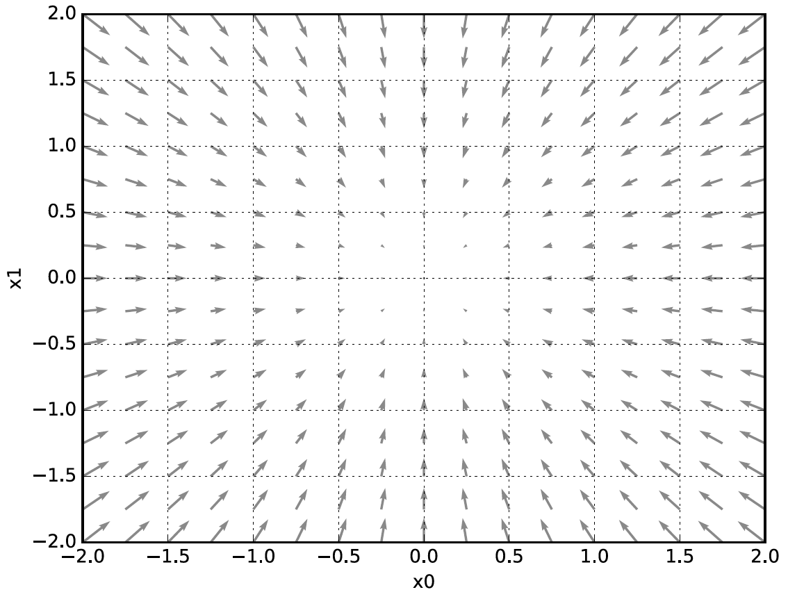
The way that arrow points is the place where decreases output value

4.4.1 Gradient Descent

Gradient Descent Formula

\[x_k = x_k - \eta\frac{\partial{f}}{\partial{x_k}}\]

eta($\eta$) is learning rate
eta is hyperparameter that we have to choose before learning

# init_x: initial starting point
# step_num: # of repeating
def gradient_descent(f, init_x, lr = 0.01, step_num = 100):
    x = init_x

    for i in range(step_num):
        grad = numerical_gradient(f, x)
        x -= lr*grad

    return x

init_x = np.array([-3.0, 4.0])
gradient_descent(function_2, init_x=init_x, lr = 0.1, step_num=100)

array([-6.11110793e-10,  8.14814391e-10])

However, too big/small learning rate($\eta$) makes result worse.

# lr=10.0 -> divergence result
init_x = np.array([-3.0, 4.0])
print(gradient_descent(function_2, init_x=init_x, lr = 10.0, step_num=100))

# lr=1e-10 -> end before finding minima
init_x = np.array([-3.0, 4.0])
print(gradient_descent(function_2, init_x=init_x, lr = 1e-10, step_num=100))

[-2.58983747e+13 -1.29524862e+12]
[-2.99999994  3.99999992]

[Warning]

Although Gradient Descent is the method that we mostly use in NN, this method have some problems.

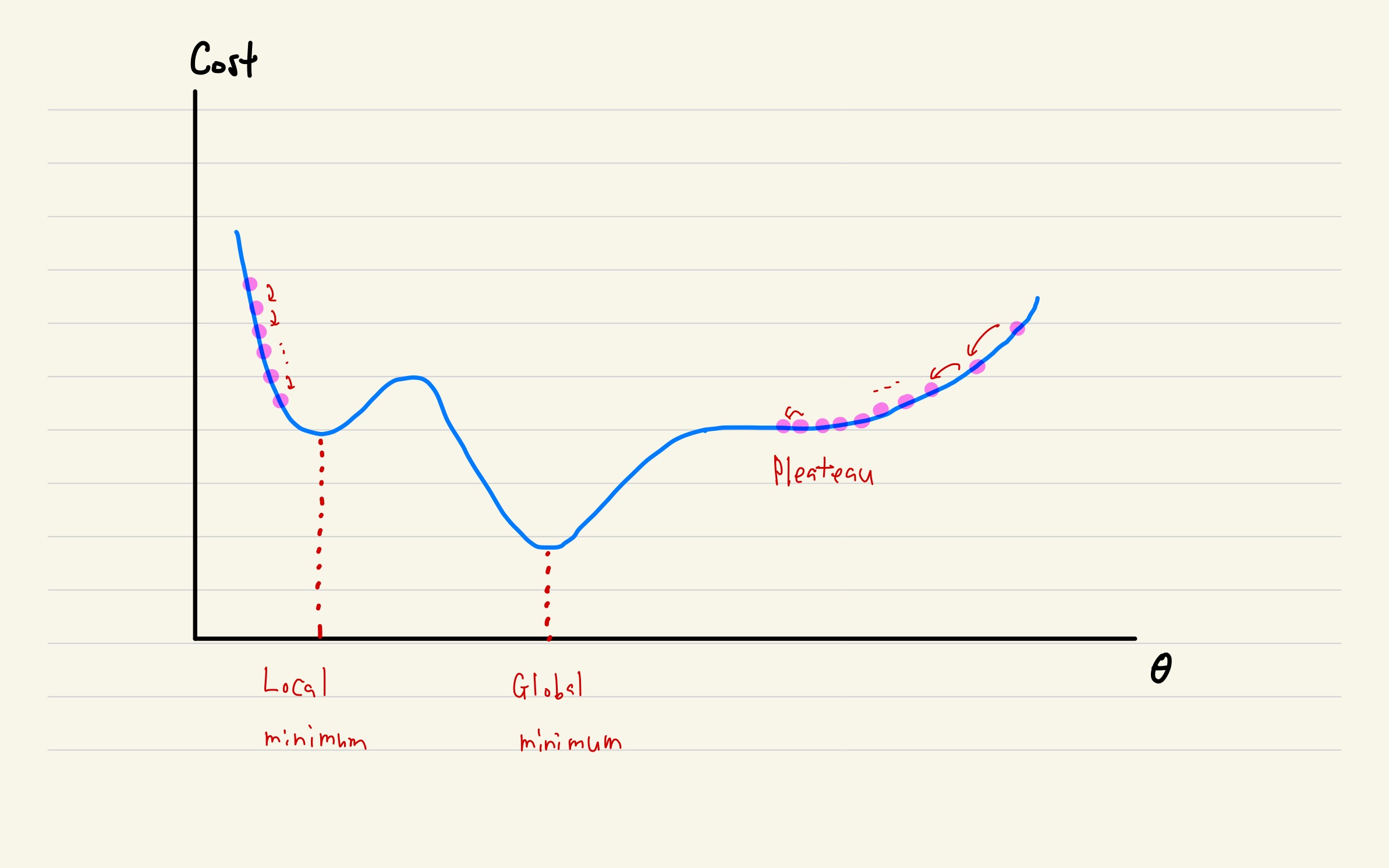
Depend on where does initial point start, it might not find Global Minimum and fall into Local Minimum
If $x_k$ fall into plateau, $x_k$ will not change anymore.

4.4.2 Gradient in Neural Network

np.random.randn(2,3)

array([[ 1.21459253,  1.04298629, -1.94374167],
       [-1.23122761,  0.83878158,  0.26981768]])

import sys, os
sys.path.append(os.pardir) # load parent directory of this ipynb file
from common.functions import softmax, cross_entropy_error
from common.gradient import numerical_gradient

class simpleNet:
    def __init__(self):
        self.W = np.random.randn(2,3) # initialize to 2x3 shape normal distribution

    def predict(self, x):
        return np.dot(x, self.W)

    def loss(self, x, t):
        z = self.predict(x)
        y = softmax(z)
        loss = cross_entropy_error(y, t)

        return loss

net = simpleNet()
print(net.W) # weight parameter

x = np.array([0.6, 0.9])
p = net.predict(x)
print(p)

print(np.argmax(p))

t = np.array([0, 0, 1])
print(net.loss(x, t))

[[ 1.78188867 -1.60339216 -1.83076049]
 [-0.27388719  0.9192118  -0.79033481]]
[ 0.82263473 -0.13474467 -1.80975762]
0
3.0079485436571267

def f(W):
    return net.loss(x, t)

numerical_gradient(f, net.W)

array([[ 0.4121426 ,  0.15822056, -0.57036316],
       [ 0.6182139 ,  0.23733084, -0.85554475]])

4.5 Learning Algorithm

Let’s put all together that we learned before

[Process of Neural Network]

1. Get Data: Batch, Mini-Batch, Online-Learning etc.

2. Find Gradient: Find Gradient that leads to minimize loss functions

3. Renew Parameter

4.5.1 2-layer Neural Network Class

from common.gradient import numerical_gradient

class TwoLayerNet:
    def __init__(self, input_size, hidden_size, output_size, weight_init_std = 0.01):
        # initiate weight
        self.params = {}
        self.params['W1'] = weight_init_std*np.random.randn(input_size, hidden_size)
        self.params['b1'] = np.zeros(hidden_size)

        self.params['W2'] = weight_init_std*np.random.randn(hidden_size, output_size)
        self.params['b2'] = np.zeros(output_size)

    def predict(self, x):
        W1, W2 = self.params['W1'], self.params['W2']
        b1, b2 = self.params['b1'], self.params['b2']

        a1 = np.dot(x, W1) + b1
        z1 = sigmoid(a1)
        a2 = np.dot(z1, W2) + b2
        y = softmax(a2)

        return y

    def loss(self, x, t):
        y = self.predict(x)

        return cross_entropy_error(y, t)

    def accuracy(self, x, t):
        y = self.predict(x)
        y = np.argmax(y, axis=1)
        t = np.argmax(t, axis=1)

        accuracy = np.sum(y==t) / float(x.shape[0])
        return accuracy

    def numerical_gradient(self, x, t):
        loss_W = lambda W: self.loss(x, t)

        # grads: contain weights
        grads = {}
        grads['W1'] = numerical_gradient(loss_W, self.params['W1'])
        grads['b1'] = numerical_gradient(loss_W, self.params['b1'])
        grads['W2'] = numerical_gradient(loss_W, self.params['W2'])
        grads['b2'] = numerical_gradient(loss_W, self.params['b2'])

        return grads

Sometimes, what value we use for initializing parameter determines the success of learning

4.5.2 mini-batch learning

from dataset.mnist import load_mnist
from two_layer_net import TwoLayerNet

(x_train, t_train), (x_test, t_test) = load_mnist(normalize=True, one_hot_label=True)

train_loss_list = []

iters_num = 10000 # iteration number
train_size = x_train.shape[0] # number of data
batch_size = 100
learning_rate = 0.1

network = TwoLayerNet(input_size=784, hidden_size=50, output_size=10)

for i in range(iters_num):
    # get mini-batch
    batch_mask = np.random.choice(train_size, batch_size)
    x_batch = x_train[batch_mask]
    t_batch = t_train[batch_mask]

    # gradient
    # grad = network.numerical_gradient(x_batch, t_batch)
    grad = network.gradient(x_batch, t_batch) # covers on next chapter.

    # renew parameter
    for key in ('W1', 'b1', 'W2', 'b2'):
        network.params[key] -= learning_rate*grad[key]

    loss = network.loss(x_batch, t_batch)
    train_loss_list.append(loss)

4.5.3 Evaluate with Test Data

from dataset.mnist import load_mnist
from two_layer_net import TwoLayerNet

(x_train, t_train), (x_test, t_test) = load_mnist(normalize=True, one_hot_label=True)

iters_num = 10000 # iteration number
train_size = x_train.shape[0] # number of data
batch_size = 100
learning_rate = 0.1

train_loss_list = []
train_acc_list = []
test_acc_list = []

iter_per_epoch = max(train_size / batch_size, 1)

network = TwoLayerNet(input_size=784, hidden_size=50, output_size=10)

for i in range(iters_num):
    # get mini-batch
    batch_mask = np.random.choice(train_size, batch_size)
    x_batch = x_train[batch_mask]
    t_batch = t_train[batch_mask]

    # gradient
    # grad = network.numerical_gradient(x_batch, t_batch)
    grad = network.gradient(x_batch, t_batch)

    # renew parameter
    for key in ('W1', 'b1', 'W2', 'b2'):
        network.params[key] -= learning_rate*grad[key]

    loss = network.loss(x_batch, t_batch)
    train_loss_list.append(loss)

    # accuracy per 1 epoch
    if i%iter_per_epoch == 0:
        train_acc = network.accuracy(x_train, t_train)
        test_acc = network.accuracy(x_test, t_test)
        train_acc_list.append(train_acc)
        test_acc_list.append(test_acc)
        print('train acc, test acc | ' + str(train_acc) + ', ' +str(test_acc))

train acc, test acc | 0.0986, 0.0957
train acc, test acc | 0.7932333333333333, 0.7953
train acc, test acc | 0.8764166666666666, 0.8794
train acc, test acc | 0.8994666666666666, 0.902
train acc, test acc | 0.9094333333333333, 0.9106
train acc, test acc | 0.9149333333333334, 0.9164
train acc, test acc | 0.9207833333333333, 0.9211
train acc, test acc | 0.9244666666666667, 0.9241
train acc, test acc | 0.9276666666666666, 0.9295
train acc, test acc | 0.9314833333333333, 0.932
train acc, test acc | 0.9344666666666667, 0.9355
train acc, test acc | 0.9368333333333333, 0.9371
train acc, test acc | 0.9388833333333333, 0.9383
train acc, test acc | 0.9412166666666667, 0.9405
train acc, test acc | 0.9432666666666667, 0.9432
train acc, test acc | 0.94555, 0.9426
train acc, test acc | 0.9474333333333333, 0.9454

Share on

Twitter Facebook LinkedIn

Philip Cho